What Is RSI?
RSI, or the Relative Strength Index, came into play in 1978 through J. Welles Wilder’s book “New Concepts in Technical Trading Systems.” Think of RSI as your financial guide, helping you navigate the world of technical analysis. It works within a range from 0 to 100, smartly checking how fast and big prices are moving for a specific thing you’re looking at.
When RSI goes over 70, it means things might be a bit too high; on the flip side, if it drops below 30, it suggests things might be a bit too low (though sometimes that’s not the case). This cool tool gives traders a peek into how the market is moving, giving them useful clues about possible changes and how strong trends are.
Traders commonly rely on RSI to identify market conditions, with readings above 70 suggesting an overbought market and readings below 30 indicating an oversold market (though exceptions may exist). This dynamic indicator, offering insights into the strength and potential reversals in price trends, has become an integral tool for traders navigating the complexities of financial markets. So in our post titled RSI Explained: Calculation and Backtesting RSI Trading Strategy we will do the following things:
Calculations Behind RSI:
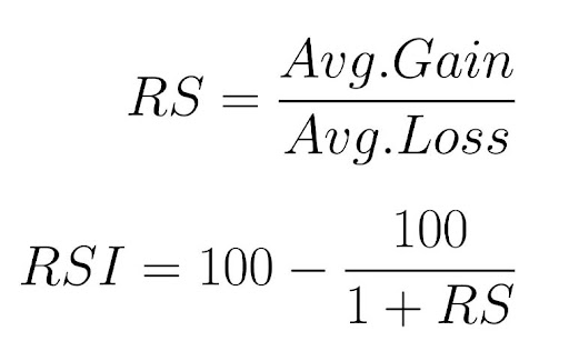
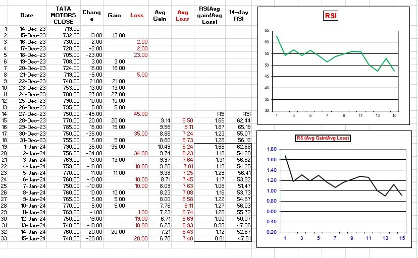
The Relative Strength Index (RSI) has three main parts: RS(Relative Strength), Average Gain, and Average Loss. It’s calculated over 14 periods, as suggested by Wilder. The first Average Gain and Average Loss are simple averages of gains and losses over the past 14 periods.
- First Average Gain = Sum of Gains in the last 14 periods / 14
- First Average Loss = Sum of Losses in the last 14 periods / 14
The next calculations use the previous averages and the current gain or loss(like on the next calculation it will skip the one row because it will become 15 periods older and we need 14 periods):
- Average Gain = [(previous Average Gain) x 13 + current Gain] / 14
- Average Loss = [(previous Average Loss) x 13 + current Loss] / 14
This method smoothens the values, like an exponential moving average, and becomes more accurate with more data points. TradingView uses at least 250 data points for RSI calculations.
Wilder’s formula normalizes RS, making RSI an oscillator ranging from 0 to 100. When the Average Gain is zero, the RSI is zero, indicating prices consistently moved lower. RSI is 100 when the Average Loss is zero, showing prices consistently moved higher. This normalization helps identify extremes in RSI as it stays within a set range.
Below is the template for calculating RSI in Excel. You can download the sheet here[RSI-Calc].
Common RSI Trading Strategy:
The strategy is straightforward: initiate a buy when the RSI surpasses 70, indicating potentially overbought conditions, and execute a sell when the RSI dips below 30, signalling potentially oversold conditions. But we’re not stopping there. To fortify our strategy, we’re incorporating an ATR-based Stop Loss, adding an extra layer of risk management.
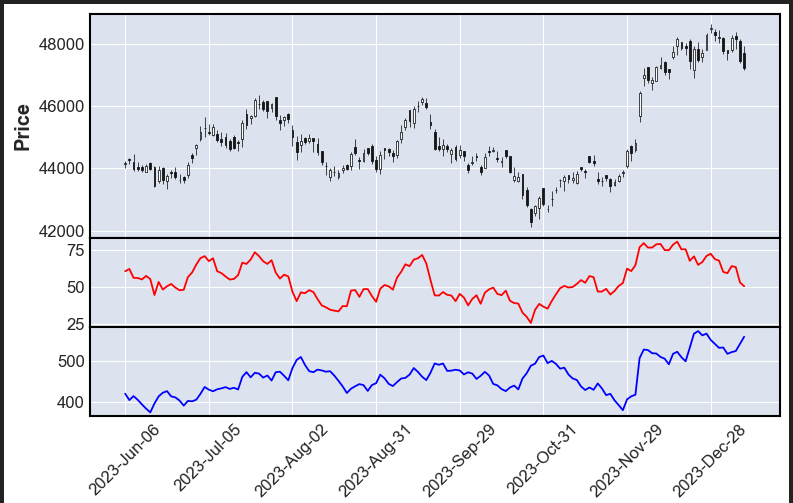
The image below Shows Our CandleStick Chart With RSI and ATR Values.
Getting Historical Data & Setting UP RSI & ATR in Python:
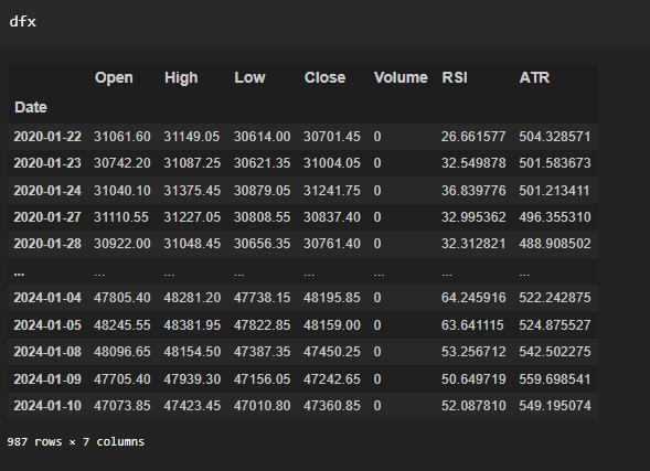
To Start backtesting an RSI trading strategy in Python, the first essential step is to gather historical data for our selected trading symbol. In this case, I’m utilizing the NIFTY BANK daily data spanning the past four years. The tool of choice for calculating the RSI and ATR is the pandas_ta library, adding a layer of efficiency and convenience to our analysis. The Python code used and the Data Shown Below.
					import pandas_ta as ta
import numpy as np
import datetime
data = historical_data('NIFTY BANK',"2020-01-01 09:15:00", "2024-01-10 15:30:00", "day")
data["RSI"] = ta.rsi(data.close, length=14)
data["ATR"] = ta.atr(data.high,data.low,data.close, length=14)
After executing the code snippet, our data will take on the following appearance:
Backtesting RSI strategy With Python :
We’ll Use a Python for loop to conduct a backtest for our RSI trading strategy. A long signal will be triggered when the price surpasses the 70 mark, while a short signal will be initiated upon crossing below 30. To ensure the effectiveness of our strategy, we’ll carefully monitor the previous RSI value, ensuring that consecutive signals are avoided by comparing it with the current candle RSI. We will use STOPLOSS as our current ATR and TARGET as twice of ATR.
Full Backtesting Code is available Below With all the relevant Information In comments. This code is ready to use you can use it in your environment to backtest your RSI-based strategy.
					capital = 100000 #initial capital
slippage = 0  #slippage
signal = ""
trd = pd.DataFrame(columns=["Signal", "Entry time", "Buy Price", "Quantity", "Exit time", "Sell price", 'Points', "Profit", "Capital"])
#trd is empty df to record trades
cur_cap = capital
# Iterate through dfx
for i in range(len(dfx)):
    cc = dfx.iloc[i]  #current_candle
    pc = dfx.iloc[i - 1]  #previous_candle
    cc['RSI'] > 70 and pc['RSI'] < 70
    if signal == "":
        if cc['RSI'] > 70 and pc['RSI'] < 70:
            signal = "buy"
            buy_pri = cc['Close'] + cc['Close'] * slippage
            sl = cc['Close'] - cc['ATR'] #stoploss
            tar = cc['Close'] + cc['ATR']*2  #tar is target
            entry_time = cc.name  #  'Entry time'
            print(f"{signal} {entry_time} {sl} {tar}")
            quantity = round(capital/cc['Close'])
        if cc['RSI'] < 30 and pc['RSI'] > 30:
            signal = "sell"
            sell_pri = cc['Close'] + cc['Close'] * slippage
            sl = cc['Close'] + cc['ATR']
            tar = cc['Close'] - cc['ATR']*2
            entry_time = cc.name  # Change to 'Exit time'
            quantity = round(capital/cc['Close'])
            print(f"{signal} {entry_time} {sl} {tar}")
    elif signal == "buy":
        if cc['High'] > tar:
            exit_time = cc.name  # 'Exit time'
            sq = tar  # squre off on target
            pt = sq - buy_pri  #points captured
            pro = (sq - buy_pri)*quantity #profit/loss
            cur_cap = cur_cap + pro #next equity
            trd.loc[len(trd.index)] = [signal, entry_time, buy_pri, quantity, exit_time, sq, pt, pro, cur_cap]
            signal = ""   #again signal to none
        elif cc['Low'] < sl:
            exit_time = cc.name  # 'Exit time'
            sq = sl
            pt = sq - buy_pri
            pro = (sq - buy_pri)*quantity
            cur_cap = cur_cap + pro
            trd.loc[len(trd.index)] = [signal, entry_time, buy_pri, quantity, exit_time, sq, pt, pro, cur_cap]
            signal = ""
    elif signal == "sell":
        if cc['High'] > sl:
            exit_time = cc.name  # 'Exit time'
            sq = sl
            #print(sq)
            pt = sell_pri - sq
            pro = (sell_pri - sq)*quantity
            cur_cap = cur_cap + pro
            trd.loc[len(trd.index)] = [signal, entry_time, sell_pri, quantity, exit_time, sq, pt, pro, cur_cap]
            signal = ""
        elif cc['Low'] < tar:
            exit_time = cc.name  # 'Exit time'
            sq = tar
            pt = sell_pri - sq
            pro = (sell_pri - sq)*quantity
            cur_cap = cur_cap + pro
            trd.loc[len(trd.index)] = [signal, entry_time, sell_pri, quantity, exit_time, sq, pt, pro, cur_cap]
            signal = ""
When We Run the above code we will receive our TradeLogs in trd DataFrame Initiated By Us in the beginning. above code will help us backtest our RSI Trading Strategy In Python.
Resulting TradeLogs Shown Below:
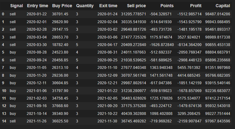
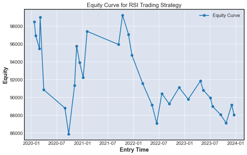
While the initial trade logs indicate a consistent loss for this strategy on the current instrument, it’s important to note that this doesn’t mark the end of our approach with the RSI indicator. There are alternative avenues to explore its effectiveness, such as incorporating divergences or leveraging it in conjunction with other indicators. This adaptive approach allows us to refine and enhance our signals, opening up possibilities for more robust and successful trading strategies.
Conclusion:
In conclusion, this post aimed to explain the Relative Strength Index (RSI) by clearly understanding its concept and demonstrating how to calculate it using Excel. We delved into the practical application of the RSI through a step-by-step guide on backtesting a trading strategy using Python. By showcasing the implementation of the RSI trading strategy, we empowered readers to explore and optimize their approaches in the dynamic world of financial markets.
If you’re interested in further enhancing your algorithmic trading skills, take advantage of our previous post, where we explored the intricacies of backtesting an Exponential Moving Average (EMA) crossover strategy using Python. Discover the diverse possibilities of algorithmic trading and deepen your insights by checking out the post.
Happy trading and may your strategies be ever profitable!

