Bollinger Bands are one of the most popular technical analysis tools used by traders to identify overbought and oversold conditions in the market. This tutorial will walk you through the process of implementing Bollinger Bands in Python using the pandas_ta library and visualizing them using mplfinance.
Brief History of Bollinger Bands
Bollinger Bands were developed by John Bollinger in the 1980s. John Bollinger, a financial analyst and an author, created this tool to provide a relative definition of high and low prices. According to Bollinger, prices are high at the upper band and low at the lower band. The width of the bands is determined by the volatility of the market; they expand when the market is volatile and contract when the market is less volatile.
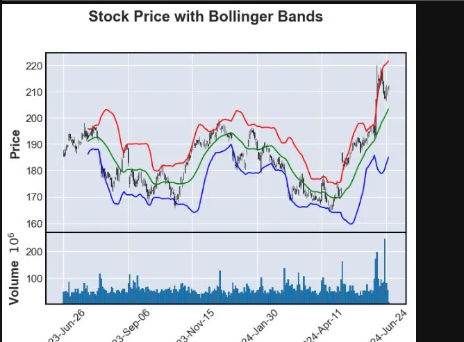
Bollinger Bands consist of three lines:
- Middle Band: This is a simple moving average (SMA) of the price, usually set to a 20-day period.
- Upper Band: This is the middle band plus two standard deviations.
- Lower Band: This is the middle band minus two standard deviations.
The bands help traders determine whether prices are high or low on a relative basis, providing a dynamic and adaptive way to assess price action.
Prerequisites
Before we start, ensure you have the necessary libraries installed. You can install them using pip:
pip install pandas pandas_ta mplfinance
Pandas is a powerful open-source data analysis and manipulation library for Python, offering robust data structures and functions for handling structured data seamlessly (pip install pandas). Pandas TA (Technical Analysis) is an extension built on top of Pandas, providing over 130 technical analysis indicators and utility functions for tasks like moving averages and oscillators (pip install pandas_ta). mplfinance is a library tailored for financial data visualization, enabling the easy creation of high-quality financial plots such as candlestick charts and volume bars, built on top of Matplotlib (pip install mplfinance).
Step 1: Import Libraries
					import pandas as pd
import pandas_ta as ta
import mplfinance as mpf
Step 2: Load Your Data
You need historical price data to calculate Bollinger Bands. For this example, we’ll first download an sample stock price data for ‘AAPL’ stock using yahoo finance you can use below snippet to do this.
					import pandas as pd
import yfinance as yf
from datetime import datetime
ticker = "AAPL"
end_date = datetime.now()
start_date = end_date.replace(year=end_date.year - 1)
data = yf.download(ticker, start=start_date, end=end_date)
csv_filename = "AAPL_1_year_data.csv"
data.to_csv(csv_filename)
data_from_csv = pd.read_csv(csv_filename, index_col='Date', parse_dates=True)
print(data_from_csv.head())
The Data will look like this in your Ide.
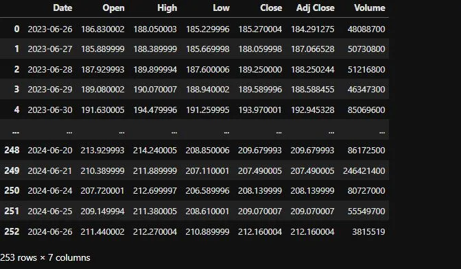
Make sure your CSV file has at least ‘Date’, ‘Open’, ‘High’, ‘Low’, ‘Close’, and ‘Volume’ columns.
Calculate Bollinger Bands
Using pandas_ta, calculating Bollinger Bands is straightforward. The default period is 20, and the standard deviation multiplier is 2.
					BB = ta.bbands(data_from_csv['Close'], length=20, std=2, ddof=0, mamode=None, talib=None, offset=None)
combined_data = pd.concat([data_from_csv, BB], axis=1)
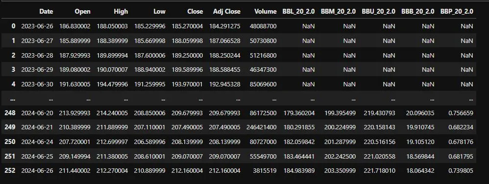
In this code snippet, we calculate Bollinger Bands for the closing prices of the stock. The bbands function returns a DataFrame with the lower, middle, and upper bands.
Here is Final Outcome of Combined_data:
Prepare Data for Visualization
mplfinance requires specific column names for the data it visualizes. We’ll rename the columns accordingly. It also requires Date as the index so we will set Date as its index.
					combined_data.set_index('Date', inplace=True)
combined_data.rename(columns={'Open': 'open', 'High': 'high', 'Low': 'low', 'Close': 'close', 'Volume': 'volume'}, inplace=True)
This step ensures that our data conforms to the format expected by mplfinance.
Visualize with mplfinance:
Now, let’s visualize the data along with Bollinger Bands.
					import mplfinance as mpf
apdict = [
    mpf.make_addplot(combined_data['BBU_20_2.0'], color='r'),
    mpf.make_addplot(combined_data['BBM_20_2.0'], color='g'),
    mpf.make_addplot(combined_data['BBL_20_2.0'], color='b')
]
# Plot the data
mpf.plot(combined_data, type='candle', addplot=apdict, volume=True, title='Stock Price with Bollinger Bands')
That’s it now after running this code you will receive output as shown in below image:
Conclusion:
In this tutorial, we implemented Bollinger Bands using the pandas_ta library and visualized them with mplfinance. Bollinger Bands are a versatile tool that can help traders identify overbought and oversold conditions and gauge market volatility.
In our next post, we will backtest a Bollinger band strategy using Python so stay tuned.
We also created a trading bot using the help of Rsi Checkout here.
Feel free to leave any questions or comments below. Happy trading!

