Backtesting Supertrend Algo Trading Strategy Using Python

Introduction to SuperTrend:

Introducing the Supertrend Algorithm:

The Supertrend algorithm is a widely-used technical indicator in financial markets, particularly in algorithmic trading strategies.
It is designed to identify trends and potential entry and exit points based on price action.
The Supertrend line is calculated using the average true range (ATR) and multiplier factors, providing dynamic support and resistance levels.

Uses of Supertrend in Trading:

Supertrend helps traders identify the direction of the trend, whether bullish or bearish, by plotting the trend line on price charts.
It generates buy signals when the price crosses above the Supertrend line and sell signals when it crosses below, indicating potential trend reversals.
Traders use Supertrend to filter out noise in price movements and focus on trading opportunities aligned with the prevailing trend.
Significance of Supertrend in Algorithmic Trading:

In algorithmic trading, where speed and precision are paramount. Supertrend is the best trend-following indicator available in the market right now.
Its straightforward calculation and clear buy/sell signals make it suitable for incorporation into automated trading bots.

You Can Read About the Supertrend Indicator here.

Data Collection For Backtesting:

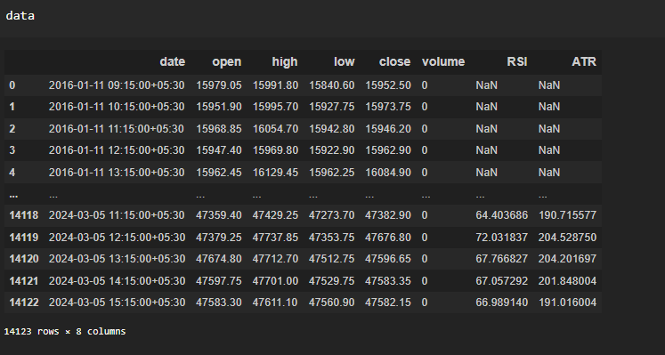
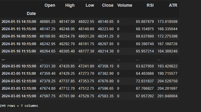
Before diving into backtesting the Supertrend strategy using Python, we need to gather the necessary data for our analysis. In this case, I’ve opted to utilize data from one of the most volatile indices in the Indian market, namely BankNifty. Below, you’ll find a glimpse of the dataset we’ll be working with.

To enhance our analysis, we’ll incorporate additional indicators such as the Relative Strength Index (RSI) and Average True Range (ATR) into the dataset. To achieve this, I’ve employed the following code, utilizing the pandas-ta library to calculate the values of these indicators.

				
					import pandas_ta as ta
import numpy as np
import datetime
data = historical_data('NIFTY BANK',"2016-01-10 09:15:00", "2024-03-05 15:30:00", "60minute")
data["RSI"] = ta.rsi(data.close, length=14)
data["ATR"] = ta.atr(data.high,data.low,data.close, length=14)

Supertrend Calculation:

We’ll Use the power of pandas-ta to compute the Supertrend indicator. The following code snippet demonstrates how we can calculate the Supertrend and visualize its impact using the image provided below. In this code, ‘sti’ represents our Supertrend indicator, and we’ll retrieve the corresponding Open, High, Low, and Close (OHLC) values from our ‘data’ variable.

				
					sti= ta.supertrend(data['high'], data['low'], data['close'], length=10, multiplier=3)

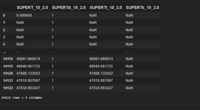
Next, we’ll merge the Supertrend data with our main dataset, ensuring to remove any NaN values in the process. The following code snippet accomplishes this task, storing the resulting data in a variable named ‘Data_True’.

				
					data = pd.merge(data, sti, left_index=True,right_index=True)
data = data[["date","open","high","low","close","volume","RSI","ATR","SUPERT_10_3.0"]]
data['date'] = data['date'].astype(str).str.split('+', expand=True)[0]
data_True = pd.DataFrame(data)
data_True.rename(columns={'date': 'Date', 'open': 'Open', 'high': 'High', 'low': 'Low', 'close': 'Close', 'volume': 'Volume'}, inplace=True)
data_True.dropna(inplace=True)
data_True.reset_index(drop=True, inplace=True)
data_True['Date'] = pd.to_datetime(data_True['Date'])
data_True = data_True.set_index('Date')

data_true response:

Strategy Visualization:

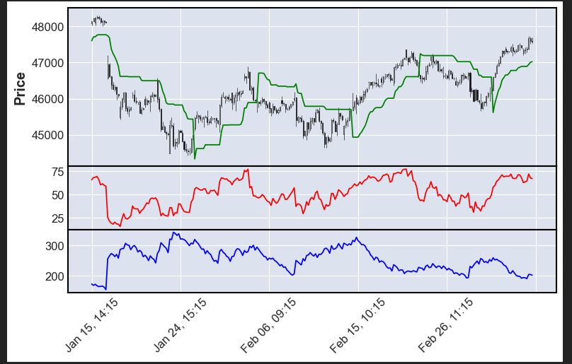
Now, let’s visualize our data using the mpl-finance library. Below, you’ll find the code snippet that leverages mpl-finance to create candlestick visualizations. This library offers powerful tools for displaying financial data in an intuitive and informative manner.

				
					dfx1 =data_True[-250:-1]
import mplfinance as mpf
adp= [mpf.make_addplot(dfx1['SUPERT_10_3.0'],type ='line',color='green'),
    mpf.make_addplot(dfx1['RSI'],type ='line',color='red',panel = 1),
     mpf.make_addplot(dfx1['ATR'],type ='line',color='blue',panel = 2)]

mpf.plot(dfx1,type='candle',figratio=(20,12),addplot=adp)

Backtesting Supertrend Algo Trading Strategy.

Variable Initialization:

capital: Represents the initial capital available for trading.
slippage: Indicates the slippage parameter, which accounts for the difference between expected and actual trade prices.
signal: Stores the current trading signal (‘buy’ or ‘sell’).
trd: Initializes an empty DataFrame to record trade details including entry and exit times, prices, quantities, profits, and capital.
cur_cap: Tracks the current capital during the trading process.

Iterating Through Data:

The code iterates through each row (candle) in the dfx DataFrame, representing the financial data.
It accesses the current candle cc and the previous candle pc for analysis.

Trading Logic:

If no signal is active (signal == ""), the code checks for conditions to initiate a trade:
- For a buy signal, if the closing price exceeds the Supertrend indicator and it’s within trading hours, a buy signal is generated.
- For a sell signal, if the closing price falls below the Supertrend indicator and it’s within trading hours, a sell signal is generated.
- Once a signal is generated, relevant trade parameters such as entry time, stop-loss (sl), target price (tar), and quantity are determined.

Handling Open Positions:

If a buy signal is active (signal == "buy"), the code monitors conditions for exiting the trade:
If the time is beyond the trading hours or the price reaches the target, the trade is closed with a sell signal.
If the price falls below the stop-loss level, the trade is exited to limit losses.
If a sell signal is active (signal == "sell"), similar exit conditions are checked.

Recording Trades:

Details of each trade, including entry and exit times, prices, quantities, profits, and updated capital, are recorded in the trd DataFrame.
The trade record is updated with each iteration, reflecting the outcome of each trade.

Output and Position Management:

The code prints trade-related information such as signals, entry times, stop-loss, and target prices for analysis.
It manages the position status (position_open) to ensure proper handling of open trades.

Conclusion of Trading:

Once the iteration through the data is complete, the code provides a summary of trades executed, including profits and updated capital.
It effectively manages trade execution based on predefined rules, incorporating the Supertrend algorithm for generating trading signals and risk management.

				
					capital = 500000 #initial capital
slippage = 0  #slippage

signal = ""  
trd = pd.DataFrame(columns=["Signal", "Entry time", "Buy Price", "Quantity", "Exit time", "Sell price", 'Points', "Profit", "Capital"])
#trd is empty df to record trades
cur_cap = capital
# Iterate through dfx
position_open=False
for i in range(len(dfx)):
    cc = dfx.iloc[i]  #current_candle
    pc = dfx.iloc[i - 1]  #previous_candle
    if signal == "":
        if cc['Close'] > cc['SUPERT_10_3.0'] and pc['Close'] < pc['SUPERT_10_3.0'] and  cc.name.time() > datetime.time(9, 18) and cc.name.time() < datetime.time(15, 0) and position_open==False  : 
            signal = "buy"
            buy_pri = cc['Close'] + cc['Close'] * slippage
            sl =   cc['SUPERT_10_3.0'] #- cc['ATR']*1.5  #cc['Close'] -cc['ATR'] *4 #stoploss
            tar = cc['Close'] +cc['ATR']*500#tar is target
            entry_time = cc.name  #  'Entry time'
            print(f"{signal} {entry_time} {sl} {tar}")
            quantity = 50#round(cur_cap / cc['Close'] / 50) * 50
            position_open=True
            
        elif cc['Close'] < cc['SUPERT_10_3.0'] and pc['Close'] > pc['SUPERT_10_3.0'] and  cc.name.time() > datetime.time(9, 18) and  cc.name.time() < datetime.time(15, 0) and position_open==False: 
            signal = "sell"
            sell_pri = cc['Close'] + cc['Close'] * slippage
            sl =  cc['SUPERT_10_3.0'] #+ cc['ATR']*1.5   #cc['Close'] +cc['ATR'] *4
            tar = cc['Close'] - cc['ATR']*500
            entry_time = cc.name  # Change to 'Exit time'
            quantity =50# round(cur_cap / cc['Close'] / 50) * 50
            print(f"{signal} {entry_time} {sl} {tar}")
            position_open=True
            
    elif signal == "buy":
        if pc['SUPERT_10_3.0']>sl:
            sl=pc['SUPERT_10_3.0']
        if cc.name.time() > datetime.time(15, 21): 
            print("sell")
            exit_time = cc.name
            sq = pc['Close']
            pt = sq - buy_pri
            pro = (sq - buy_pri)*quantity
            cur_cap = cur_cap + pro
            trd.loc[len(trd.index)] = [signal, entry_time, buy_pri, quantity, exit_time, sq, pt, pro, cur_cap]
            signal = ""
            position_open=False
        if cc['High'] > tar: 
            exit_time = cc.name  # 'Exit time'
            sq = pc['SUPERT_10_3.0']  # squre off on target
            pt = sq - buy_pri  #points captured
            pro = (sq - buy_pri)*quantity #profit/loss
            cur_cap = cur_cap + pro #next equity
            trd.loc[len(trd.index)] = [signal, entry_time, buy_pri, quantity, exit_time, sq, pt, pro, cur_cap]
            signal = ""   #again signal to none
            position_open=False
        elif cc['Low'] < sl: 
            exit_time = cc.name  # 'Exit time'
            sq = pc['SUPERT_10_3.0']
            pt = sq - buy_pri
            pro = (sq - buy_pri)*quantity
            cur_cap = cur_cap + pro
            trd.loc[len(trd.index)] = [signal, entry_time, buy_pri, quantity, exit_time, sq, pt, pro, cur_cap]
            signal = ""
            position_open=False
        
    elif signal == "sell":
        if pc['SUPERT_10_3.0']<sl:
            sl=pc['SUPERT_10_3.0']
        if cc.name.time() > datetime.time(15, 21):
            print("this")
            exit_time = cc.name
            sq = cc['Close']
            pt = sell_pri - sq
            pro = (sell_pri - sq)*quantity
            cur_cap = cur_cap + pro
            trd.loc[len(trd.index)] = [signal, entry_time, sell_pri, quantity, exit_time, sq, pt, pro, cur_cap]
            signal = ""
            position_open=False    
            
        if cc['High'] > sl: 
            exit_time = cc.name  # 'Exit time'
            sq = pc['SUPERT_10_3.0']
            #print(sq)
            pt = sell_pri - sq
            pro = (sell_pri - sq)*quantity
            cur_cap = cur_cap + pro
            trd.loc[len(trd.index)] = [signal, entry_time, sell_pri, quantity, exit_time, sq, pt, pro, cur_cap]
            signal = ""
            position_open=False
            
        elif cc['Low'] < tar: 
            exit_time = cc.name  # C'Exit time'
            sq = pc['SUPERT_10_3.0']
            pt = sell_pri - sq
            pro = (sell_pri - sq)*quantity
            cur_cap = cur_cap + pro
            trd.loc[len(trd.index)] = [signal, entry_time, sell_pri, quantity, exit_time, sq, pt, pro, cur_cap]
            signal = ""
            position_open=False

Analyzing Backtest Data:

Below is our ‘trd’ DataFrame containing all the pertinent trade data. This DataFrame serves as a comprehensive record of our trading activity, encompassing details such as entry and exit times, prices, quantities, profits, and updated capital.

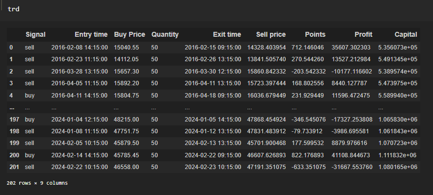
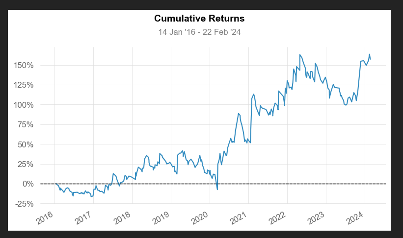
Now, let’s leverage the quantstats module to analyze our backtest performance. This powerful module allows us to calculate various performance metrics and visualize our equity curve for the strategy discussed above. I’ll demonstrate the performance matrix and the resulting equity curve, providing insights into the effectiveness of our trading strategy.

				
					import quantstats as qs

backtest = trd.set_index('Entry time')
backtest['Returns'] = backtest['Capital'].pct_change()
backtest = backtest.fillna(0)

				
					qs.reports.full(backtest['Returns'])

Conclusion:

In this guide, we explored how to backtest a Supertrend algorithmic trading bot using Python. The Supertrend algorithm, known for its simplicity and effectiveness in identifying trends, was at the core of our strategy.

By automating the process of identifying trend opportunities, we eliminated emotional biases and enhanced trading efficiency. We set up our trading environment, defined clear entry and exit rules based on Supertrend signals, and conducted thorough backtests to evaluate performance.

Our approach prioritized risk management, ensuring trades were closed based on predefined criteria to protect capital. With each trade recorded and capital updated accordingly, we maintained transparency and accountability throughout the process.

You can checkout my other posts on backtesting here.

Also Checkout Backtesting Ema crossover strategy using python.