Forex trading strategies are essential for traders aiming to capitalize on market movements. Among these, scalping is a popular method that involves making multiple trades throughout the day to profit from small price changes. This blog post will guide you through a comprehensive Forex scalping strategy using Exponential Moving Averages (EMA) and the Average True Range (ATR) indicators. We will also backtest the strategy using Python to validate its effectiveness.

Backtesting a Forex Scalping Strategy Step-BY-Step Guide:

Fetching Historical Data

To begin with, we need to fetch historical data for the EUR/USD currency pair. Using the yfinance library, we can download 15-minute interval data for the past 60 days.

				
					import pandas as pd
import yfinance as yf

ticker = "EURUSD=X"
interval = "15m"
period = "60d"
data = yf.download(ticker, period=period, interval=interval)
data.to_csv("USDEUR.csv")

This block of code downloads the historical price data and saves it to a CSV file. This data will be used to calculate the indicators necessary for our scalping strategy.

Loading and Preparing Data

				
					data_from_csv = pd.read_csv("USDEUR.csv", index_col='Datetime', parse_dates=True)
df = data_from_csv[data_from_csv['Volume'] == 0]

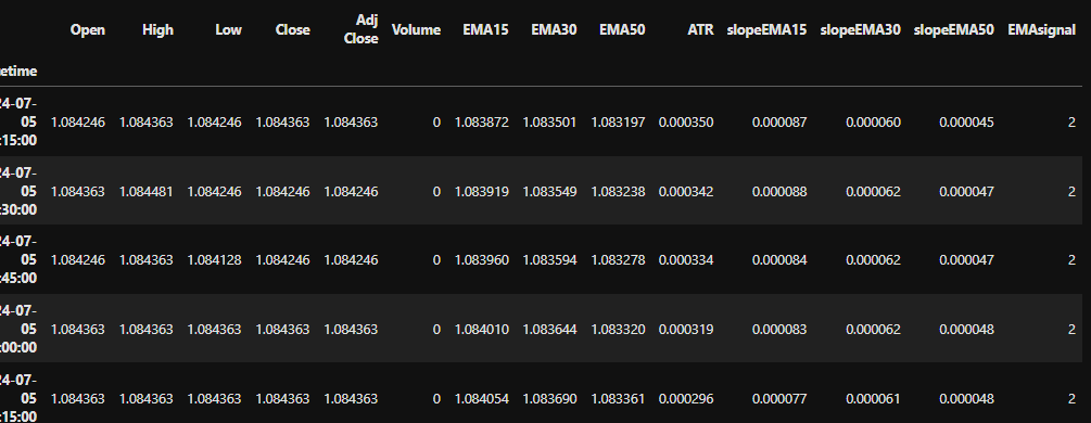
Filtering out zero-volume rows ensures that we are analyzing active trading periods, which is crucial for accurate signal generation in Forex trading strategies.

Calculating EMA and ATR Indicators

We calculate the EMA for different periods (15, 30, and 50) and the ATR to understand market volatility.

				
					import pandas_ta as ta

df["EMA15"] = ta.ema(df['Close'], length=15)
df["EMA30"] = ta.ema(df['Close'], length=30)
df["EMA50"] = ta.ema(df['Close'], length=50)
df['ATR'] = ta.atr(df['High'], df['Low'], df['Close'])

These indicators help identify the trend direction and market volatility, which are crucial for making informed trading decisions.

Generating Trading Signals

We define conditions to generate buy and sell signals based on the relative positioning and slope of the EMAs.

				
					import numpy as np

df['slopeEMA15'] = df['EMA15'].diff(periods=1).rolling(window=10).mean()
df['slopeEMA30'] = df['EMA30'].diff(periods=1).rolling(window=10).mean()
df['slopeEMA50'] = df['EMA50'].diff(periods=1).rolling(window=10).mean()

conditions = [
    (df['EMA15'] < df['EMA30']) & (df['EMA30'] < df['EMA50']) & (df['slopeEMA15'] < 0) & (df['slopeEMA30'] < 0) & (df['slopeEMA50'] < 0),
    (df['EMA15'] > df['EMA30']) & (df['EMA30'] > df['EMA50']) & (df['slopeEMA15'] > 0) & (df['slopeEMA30'] > 0) & (df['slopeEMA50'] > 0)
]

choices = [1, 2]
df['EMAsignal'] = np.select(conditions, choices, default=0)

These conditions help us identify when to enter a buy or sell position based on the alignment and trend of the EMAs, which is a key aspect of any successful Forex trading strategy.

Implementing Total Signals

We further refine the signals by considering the candle’s open and close positions relative to the EMAs and setting a wick limit to filter out noise.

				
					TotSignal = [0] * len(df)
wicklimit = 2e-5

for row in range(len(df)):
    if df['EMAsignal'][row] == 1 and df['Open'][row] > df['EMA15'][row] and df.Close[row] < df.EMA15[row] and df['High'][row] - df['Open'][row] <= wicklimit:
        TotSignal[row] = 1
    if df['EMAsignal'][row] == 2 and df['Open'][row] < df['EMA15'][row] and df.Close[row] < df.EMA15[row] and df['Open'][row] - df['Low'][row] <= wicklimit:
        TotSignal[row] = 2

df['TotSignal'] = TotSignal

This refinement helps in reducing false signals and improves the accuracy of our trading strategy.

Visualizing the Strategy

Using mplfinance, we can plot the price data along with the EMAs and generated signals.

				
					import mplfinance as mpf

def pointpos(x):
    if x['TotSignal'] == 1:
        return x['High']
    elif x['TotSignal'] == 2:
        return x['Low']
    else:
        return np.nan

df['pointpos'] = df.apply(lambda row: pointpos(row), axis=1)
df.rename(columns={'Open': 'open', 'High': 'high', 'Low': 'low', 'Close': 'close', 'Volume': 'volume'}, inplace=True)

dfpl = df[1000:1200]
apdict = [
    mpf.make_addplot(dfpl['EMA15'], color='r'),
    mpf.make_addplot(dfpl['EMA30'], color='g'),
    mpf.make_addplot(dfpl['EMA50'], color='b'),
    mpf.make_addplot(dfpl['pointpos'], type='scatter', markersize=100, marker='o', color='r')
]

mpf.plot(dfpl, type='candle', addplot=apdict, volume=True, title='EUR/USD Price with EMAs and Signals', figratio=(28, 15), style='binance')

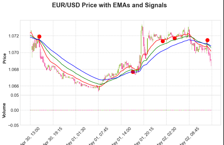
Visualizing the data helps us understand how well our strategy performs over a specific period, which is crucial for backtesting Forex strategies.

Simulating Trades

We then simulate the trading process, updating our capital based on the trades executed.

				
					capital = 2000
slippage = 0
signal = ""
trd = pd.DataFrame(columns=["Signal", "Entry time", "Buy Price", "Quantity", "Exit time", "Sell price", 'Points', "Profit", "Capital"])
cur_cap = capital
position_open = False

for i in range(len(df)):
    cc = df.iloc[i]
    if signal == "":
        if cc['TotSignal'] == 1 and not position_open:
            signal = "buy"
            buy_pri = cc['close'] + cc['close'] * slippage
            sl = cc['close'] - 30e-4
            tar = cc['close'] + 50e-4
            entry_time = cc.name
            quantity = round(cur_cap / cc['close'] / 25) * 25
            position_open = True
        elif cc['TotSignal'] == 2 and not position_open:
            signal = "sell"
            sell_pri = cc['close'] + cc['close'] * slippage
            sl = cc['close'] + 30e-4
            tar = cc['close'] - 50e-4
            entry_time = cc.name
            quantity = round(cur_cap / cc['close'] / 25) * 25
            position_open = True
    elif signal == "buy" and position_open:
        if cc['high'] > tar or cc['low'] < sl:
            exit_time = cc.name
            sq = tar if cc['high'] > tar else sl
            pt = sq - buy_pri
            pro = (sq - buy_pri) * quantity
            cur_cap = cur_cap + pro
            trd.loc[len(trd.index)] = [signal, entry_time, buy_pri, quantity, exit_time, sq, pt, pro, cur_cap]
            signal = ""
            position_open = False
    elif signal == "sell" and position_open:
        if cc['high'] > sl or cc['low'] < tar:
            exit_time = cc.name
            sq = sl if cc['high'] > sl else tar
            pt = sell_pri - sq
            pro = (sell_pri - sq) * quantity
            cur_cap = cur_cap + pro
            trd.loc[len(trd.index)] = [signal, entry_time, sell_pri, quantity, exit_time, sq, pt, pro, cur_cap]
            signal = ""
            position_open = False

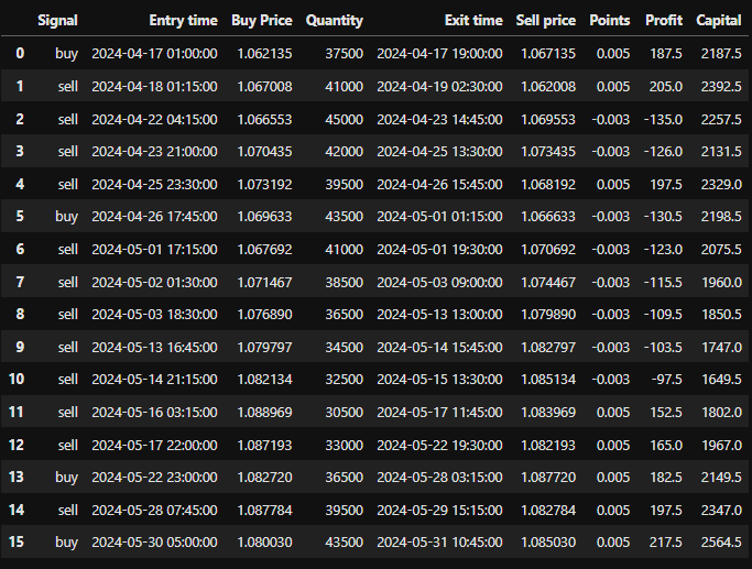
This simulation captures the entry and exit points of trades, calculates profits or losses, and updates the capital accordingly.

All the trade data will store in trd DataFrame.

Evaluating the Strategy

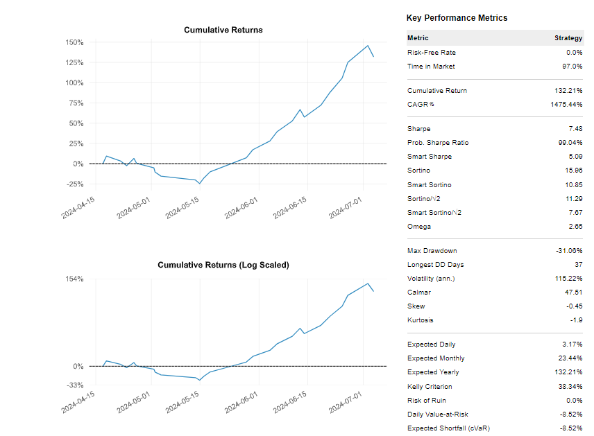
Lastly, we evaluate the strategy’s performance using quantstats.

				
					import quantstats as qs

backtest = trd.set_index('Entry time')
backtest['Returns'] = backtest['Capital'].pct_change()
backtest = backtest.fillna(0)
qs.reports.full(backtest['Returns'])

Quantstats provides a comprehensive report on the trading strategy’s performance, including key metrics such as returns, drawdowns, and various performance ratios. This evaluation is crucial to understand the effectiveness of our Forex scalping strategy.

Conclusion

In conclusion, exploring a Forex scalping strategy using EMA and ATR indicators can offer valuable insights into its potential profitability. With tools like Python and libraries such as yfinance, pandas_ta, and mplfinance, you can automate data fetching, calculate indicators, generate signals, and visualize trends. This approach involves analyzing EMA alignments and market volatility to capitalize on short-term price movements effectively.

For those eager to refine their Forex trading strategies, integrating robust backtesting methodologies is crucial. This process allows you to fine-tune strategies and make well-informed decisions, which are vital in navigating the competitive Forex landscape.

By grasping these concepts and putting them into practice, you’ll be equipped to develop and backtest your own Forex trading strategy, enhancing your ability to achieve consistent profits.

You can check our Bollinger Bands strategy backtest here.