Backtesting A Bollinger Bands Strategy Using Python

Introduction:

Bollinger Bands are a popular technical analysis tool used by traders to gauge market volatility, identify potential entry and exit points, and manage risk effectively. In our previous post, we discussed how to implement Bollinger Bands in Python using the pandas_ta library and visualize them with mplfinance. If you haven’t read it yet, you can find it here. Building upon that foundation, this comprehensive guide will walk you through the process of implementing and backtesting a Bollinger Bands trading strategy step-by-step.

In this backtesting post what we will do is Buy the ‘AAPL’ stock whenever the low is less than the lower Bollinger band and the high is greater than the lower Bollinger band & exactly the opposite for the short trade where we will sell the instrument when the high is greater than Upper Bollinger band and Low is less than Upper Bollinger Band.

Let’s get started.

Step-by-Step Implementation Guide:

Step 1: Setting Up Environment

Before proceeding, ensure you have Python installed along with necessary libraries like pandas, yfinance, pandas_ta, mplfinance, numpy, and quantstats.

				
					import pandas as pd
import yfinance as yf
from datetime import datetime
import pandas_ta as ta
import mplfinance as mpf
import numpy as np
import quantstats as qs

Step 2: Fetching Historical Data:

Fetch historical price data for the asset of interest (e.g., AAPL) using yfinance.

				
					ticker = "AAPL"
end_date = datetime.now()
start_date = end_date.replace(year=end_date.year - 5)

data = yf.download(ticker, start=start_date, end=end_date)

csv_filename = "AAPL_5_year_data.csv"
data.to_csv(csv_filename)

data_from_csv = pd.read_csv(csv_filename, index_col='Date', parse_dates=True)
print(data_from_csv.head())

Step 3: Calculating Bollinger Bands

Use pandas_ta to calculate Bollinger Bands based on the closing prices of the stock.

These step we have done in our previous post so we are not explaining it here.

				
					BB = ta.bbands(data_from_csv['Close'], length=20, std=2, ddof=0, mamode=None, talib=None, offset=None)
combined_data = pd.concat([data_from_csv, BB], axis=1)
combined_data.rename(columns={'Open': 'open', 'High': 'high', 'Low': 'low', 'Close': 'close', 'Volume': 'volume'}, inplace=True)

Step 4: Generating Trading Signals

Generate buy and sell signals based on Bollinger Bands thresholds.

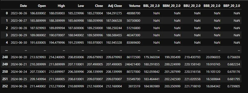
our combined_data format is like explained in the previous post.

				
					combined_data['Long_Signal'] = np.nan
combined_data['Short_Signal'] = np.nan

combined_data.loc[(combined_data['high'] > combined_data['BBU_20_2.0']) & (combined_data['low'] < combined_data['BBU_20_2.0']), 'Long_Signal'] = combined_data['high']
combined_data.loc[(combined_data['low'] < combined_data['BBL_20_2.0']) & (combined_data['high'] > combined_data['BBL_20_2.0']), 'Short_Signal'] = combined_data['high']

The Final DataFrame will look like this:

Step 5: Visualizing Signals with mplfinance:

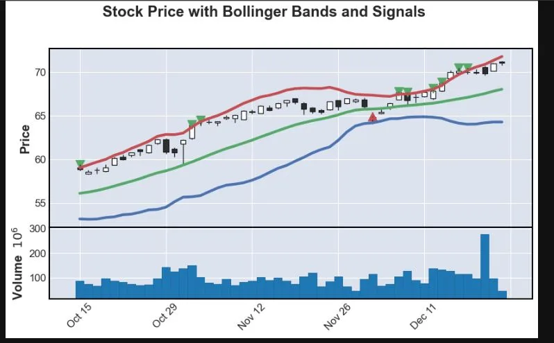
Visualize buy and sell signals alongside Bollinger Bands using mplfinance.

we will use a fraction of data to plot so we can check how our signals are generating.

				
					combined_data_plot = combined_data[75:150]

apdict = [
    mpf.make_addplot(combined_data_plot['BBU_20_2.0'], color='r'),
    mpf.make_addplot(combined_data_plot['BBM_20_2.0'], color='g'),
    mpf.make_addplot(combined_data_plot['BBL_20_2.0'], color='b'),
    mpf.make_addplot(combined_data_plot['Long_Signal'], type='scatter', markersize=100, marker='v', color='g'),
    mpf.make_addplot(combined_data_plot['Short_Signal'], type='scatter', markersize=100, marker='^', color='r')
]

mpf.plot(combined_data_plot, type='candle', addplot=apdict, volume=True, title='AAPL Stock Price with Bollinger Bands and Signals')

Step 6: Backtesting the Strategy:

Initialization:
- capital: Represents the initial amount of capital available for trading.
- slippage: Normally refers to the difference between the expected price of a trade and the actual price at which it is executed, although it’s set to zero in this example.
- signal: Variable to indicate whether a buy ("buy") or sell ("sell") signal has been triggered.
- trd: A DataFrame initialized to record trade details such as signal type, entry and exit times, prices, profits, and updated capital.
- cur_cap: Tracks the current capital throughout the backtesting process.
- position_open: Flag to indicate if there is currently an open position in the market.
Iterating through Historical Data:
- The loop iterates through each row (or candle) in the combined_data DataFrame, which contains historical price data and signals.
Generating Signals:
- Signals ("Long_Signal" and "Short_Signal") are generated based on predefined conditions derived from Bollinger Bands signals (BBU_20_2.0, BBM_20_2.0, BBL_20_2.0).
Calculating Prices:
- buy_pri and sell_pri are calculated considering slippage, representing the price at which a buy or sell trade is initiated.
- sl and tar denote the stop-loss and target prices respectively, used for risk management and profit-taking.
Managing Open Positions and Executing Trades:
- Depending on whether a long ("buy") or short ("sell") position is open (position_open), the loop checks if the price has reached the target or stop-loss levels to execute trades.
- Profit or loss (pro) is calculated based on the difference between entry and exit prices multiplied by the quantity (quantity).

Here is the code for our backtesting:

				
					
dfx = combined_data
capital = 2000#initial capital
slippage = 0  #slippage

signal = ""  
trd = pd.DataFrame(columns=["Signal", "Entry time", "Buy Price", "Quantity", "Exit time", "Sell price", 'Points', "Profit", "Capital"])
#trd is empty df to record trades
cur_cap = capital
# Iterate through dfx
position_open=False
for i in range(len(dfx)):
    cc = dfx.iloc[i]  #current_candle
    pc = dfx.iloc[i - 1]  #previous_candle
    if signal == "":
        if cc['Long_Signal'] != None and position_open==False : 
            signal = "buy"
            buy_pri = cc['close'] + cc['close'] * slippage
            sl =   cc['close'] - 2  #cc['Close'] -cc['ATR'] *4 #stoploss
            tar = cc['close'] + 10 #tar is target
            entry_time = cc.name  #  'Entry time'
            print(f"{signal} {entry_time} {sl} {tar}")
            quantity = 25#round(cur_cap / cc['Close'] / 25) * 25
            position_open=True
            
        elif cc['Short_Signal'] != None and position_open==False :
            signal = "sell"
            sell_pri = cc['close'] + cc['close'] * slippage
            sl =  cc['close'] +2  #cc['Close'] +cc['ATR'] *4
            tar = cc['close'] -10
            entry_time = cc.name  # Change to 'Exit time'
            quantity =25#round(cur_cap / cc['Close'] / 25) * 25
            print(f"{signal} {entry_time} {sl} {tar}")
            position_open=True
            
    elif signal == "buy" and position_open==True:
        if cc['high'] > tar: 
            exit_time = cc.name  # 'Exit time'
            sq = tar  # squre off on target
            pt = sq - buy_pri  #points captured
            pro = (sq - buy_pri)*quantity #profit/loss
            cur_cap = cur_cap + pro #next equity
            trd.loc[len(trd.index)] = [signal, entry_time, buy_pri, quantity, exit_time, sq, pt, pro, cur_cap]
            signal = ""   #again signal to none
            position_open=False
        elif cc['low'] < sl: 
            exit_time = cc.name  # 'Exit time'
            sq = sl
            pt = sq - buy_pri
            pro = (sq - buy_pri)*quantity
            cur_cap = cur_cap + pro
            trd.loc[len(trd.index)] = [signal, entry_time, buy_pri, quantity, exit_time, sq, pt, pro, cur_cap]
            signal = ""
            position_open=False
        
    elif signal == "sell" and position_open==True:
        if cc['high'] > sl: 
            exit_time = cc.name  # 'Exit time'
            sq = sl
            #print(sq)
            pt = sell_pri - sq
            pro = (sell_pri - sq)*quantity
            cur_cap = cur_cap + pro
            trd.loc[len(trd.index)] = [signal, entry_time, sell_pri, quantity, exit_time, sq, pt, pro, cur_cap]
            signal = ""
            position_open=False
            
        elif cc['low'] < tar: 
            exit_time = cc.name  # C'Exit time'
            sq = tar
            pt = sell_pri - sq
            pro = (sell_pri - sq)*quantity
            cur_cap = cur_cap + pro
            trd.loc[len(trd.index)] = [signal, entry_time, sell_pri, quantity, exit_time, sq, pt, pro, cur_cap]
            signal = ""
            position_open=False

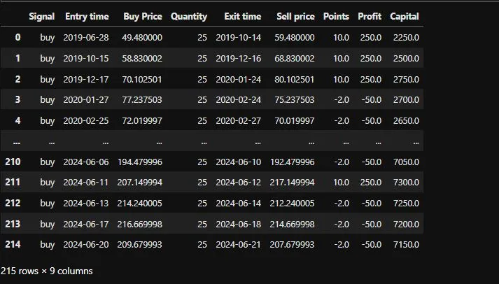
After this our trd DataFrame will look like this:

Step 7: Analyzing Backtest Results with quantstats

Utilize quantstats to analyze and visualize the backtest results, including performance metrics and equity curve.

				
					backtest = trd.set_index('Entry time')
backtest['Returns'] = backtest['Capital'].pct_change()
backtest = backtest.fillna(0)
qs.reports.full(backtest['Returns'])

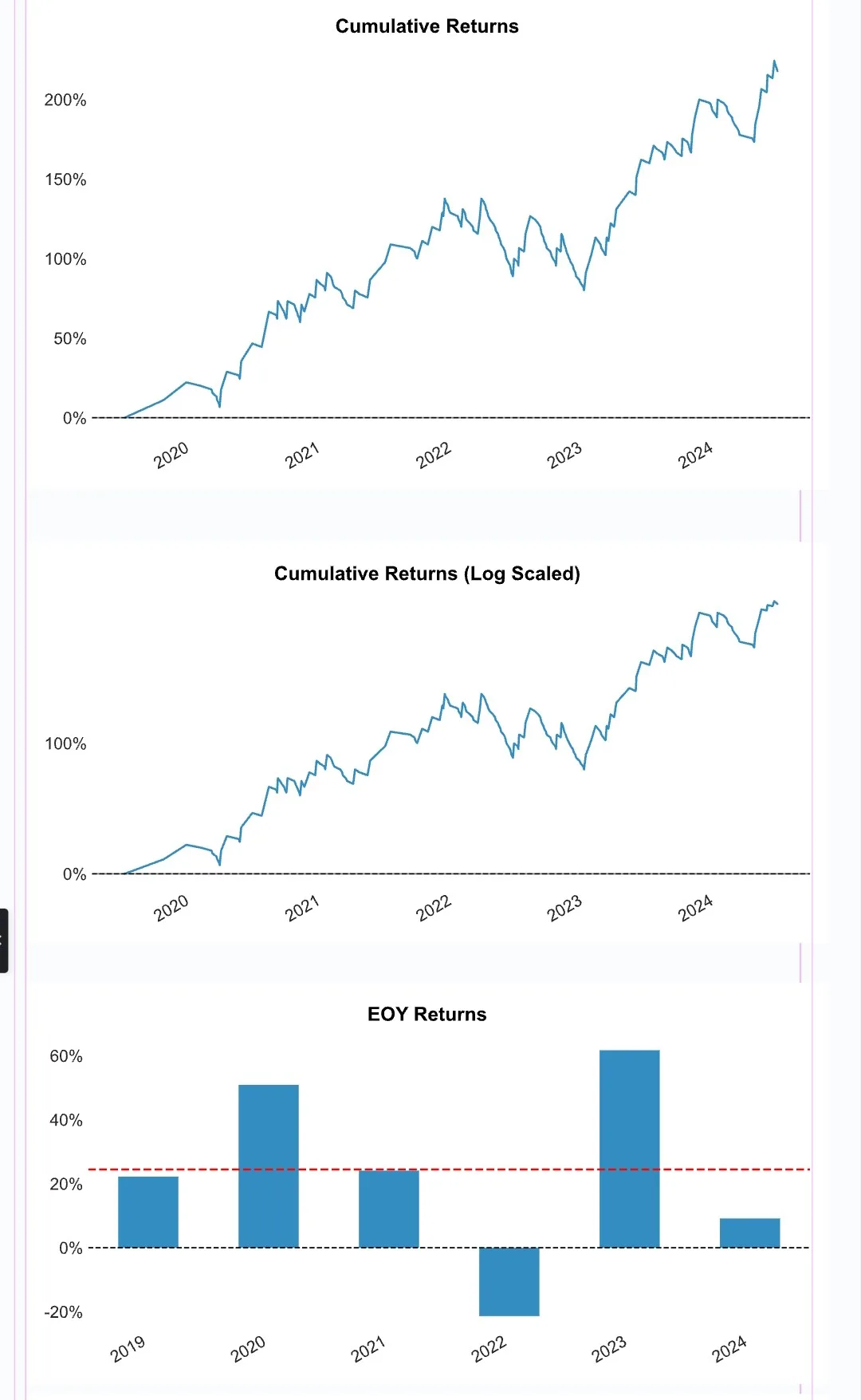
The Full Report for this stratgey is available below.

You can download the full strategy tear sheet from here.

Conclusion:

In this comprehensive guide, we have walked through the process of implementing and backtesting a Bollinger Bands trading strategy in Python. Starting with setting up your environment and fetching historical data, to calculating Bollinger Bands, generating trading signals, visualizing results, and analyzing performance metrics using quantstats, each step has been thoroughly explained.

By backtesting the strategy, traders can gain valuable insights into its historical performance, identify potential areas of improvement, and assess its viability for live trading. quantstats provides powerful tools for evaluating trading strategies, making it easier to make informed decisions based on statistical measures and risk-adjusted returns.

For more details on implementing Bollinger Bands using pandas_ta and visualizing them with mplfinance, refer to our previous post here.

Explore further and enhance your quantitative trading skills with Python. Feel free to leave any questions or comments below. Happy trading!