Supercharging RSI with AI: Building an AI Trading Indicator
Introduction
Trading strategies based on technical indicators like the Relative Strength Index (RSI) have been the foundation of many successful trading systems. However, despite its popularity, RSI, a momentum oscillator, has limitations due to its fixed thresholds and lagging nature. The solution? Enhance RSI with AI and machine learning to generate smarter, adaptive trading signals that can respond to real-time market conditions.

In this guide, we’ll walk you through the process of building an AI Trading Indicator by enhancing an RSI trading strategy using Python, TensorFlow, and LSTM (Long Short-Term Memory) neural networks. The goal is to compare the performance of a traditional RSI strategy against an AI-powered strategy to see if artificial intelligence can outperform classic technical indicators.
Understanding RSI: The Traditional Strategy
The Relative Strength Index (RSI) is a widely-used momentum oscillator that measures the speed and change of price movements. The standard RSI formula calculates a value between 0 and 100, with overbought conditions signaled when RSI > 70 and oversold conditions when RSI < 30. Traders use these levels to identify potential buy or sell opportunities. However, RSI does not adjust dynamically to varying market conditions, which can result in delayed or inaccurate signals.
Enhancing RSI with AI
The solution to the limitations of traditional RSI is to introduce AI into the decision-making process. By leveraging machine learning, specifically Long Short-Term Memory (LSTM) networks, we can enhance the RSI strategy by allowing the model to learn patterns from past data and make predictions that adapt to the current market environment.
The approach starts by calculating the RSI values for a given stock (Apple, in this case) over a specified time period. Then, we train an LSTM model to predict whether the RSI is signaling a buy, sell, or hold action based on the market’s historical behavior.
Building the AI Trading Indicator Strategy
Let’s walk through the steps involved in creating the AI-powered trading strategy:
Step 1: Fetching Historical Data
The first step is to gather historical stock data, which can be obtained from the Yahoo Finance API using the Python package `yfinance`. For our example, we will fetch the Apple stock data (AAPL) for the years 2020 to 2023.
import yfinance as yf
import pandas as pd
import numpy as np

# Fetch AAPL data
data = yf.download("AAPL", start="2020-01-01", end="2023-01-01")
Step 2: Calculating RSI
The next step is to calculate the RSI values using the formula described earlier. We will use a rolling window of 14 periods to calculate the average gains and losses and derive the RSI.
def calculate_rsi(data, window=14):
    delta = data['Close'].diff()
    gain = delta.where(delta > 0, 0)
    loss = -delta.where(delta < 0, 0)

    avg_gain = gain.rolling(window).mean()
    avg_loss = loss.rolling(window).mean()

    rs = avg_gain / avg_loss
    rsi = 100 - (100 / (1 + rs))
    return rsi

data['RSI'] = calculate_rsi(data)
Step 3: Generating Trading Signals
Next, we generate buy and sell signals based on traditional RSI thresholds. A buy signal occurs when RSI is below 40, and a sell signal is triggered when RSI exceeds 60. We also calculate the daily returns based on these signals.
data['Traditional_Signal'] = 0
data.loc[data['RSI'] < 40, 'Traditional_Signal'] = 1  # Buy signal
data.loc[data['RSI'] > 60, 'Traditional_Signal'] = -1  # Sell signal

data['Traditional_Returns'] = data['Close'].pct_change() * data['Traditional_Signal'].shift(1)
data['Traditional_Cumulative'] = (1 + data['Traditional_Returns']).cumprod()
Step 4: Preparing Data for LSTM
To train our AI model, we need to prepare the data. We create a sliding window of the past 20 RSI values to use as input features for the LSTM model. The labels for the model are based on future RSI values: if the RSI is below 40, it's labeled as a buy (2), if above 60, it's labeled as a sell (0), and in-between values are labeled as hold (1).
from sklearn.preprocessing import MinMaxScaler
from tensorflow.keras.models import Sequential
from tensorflow.keras.layers import LSTM, Dense

# Prepare dataset for LSTM
window_size = 20
X, y = [], []

# Use RSI values as input features
for i in range(window_size, len(data)):
    X.append(data['RSI'].iloc[i-window_size:i].values)
    next_day_rsi = data['RSI'].iloc[i]
    if next_day_rsi < 40:
        y.append(2)  # Buy (will be converted back to 1 for signals)
    elif next_day_rsi > 60:
        y.append(0)  # Sell (will be converted back to -1 for signals)
    else:
        y.append(1)  # Hold (will be converted back to 0 for signals)

X = np.array(X).reshape(-1, window_size, 1)  # Reshape for LSTM input
y = np.array(y)
Step 5: Training the LSTM Model
With the data prepared, we split it into training and testing sets and train an LSTM model. The LSTM is designed to predict whether the next trading signal should be a buy, sell, or hold based on the past 20 periods of RSI data.
split = int(0.85 * len(X))
X_train, X_test = X[:split], X[split:]
y_train, y_test = y[:split], y[split:]

# Create and train LSTM model
model = Sequential()
model.add(LSTM(64, return_sequences=True, input_shape=(window_size, 1)))
model.add(LSTM(32))
model.add(Dense(3, activation='softmax'))

model.compile(optimizer='adam',
              loss='sparse_categorical_crossentropy',
              metrics=['accuracy'])

history = model.fit(X_train, y_train,
                    epochs=50,
                    batch_size=32,
                    validation_split=0.2,
                    verbose=1)
Step 6: Predicting Signals and Calculating AI Strategy Returns
Once the model is trained, we can use it to predict future signals for the test set. The model will output a probability distribution for buy, hold, or sell, and we’ll convert these predictions into trading signals. We can then calculate the returns based on these AI Trading Indicator-generated signals and compare them with the traditional strategy.
# Predict using the LSTM model
y_pred = model.predict(X_test)
predicted_labels = np.argmax(y_pred, axis=1)

# Convert predictions back to trading signals (-1, 0, 1)
signal_conversion = {0: -1, 1: 0, 2: 1}
predicted_signals = np.array([signal_conversion[label] for label in predicted_labels])

# Assign AI signals to the test period
test_dates = data.index[split + window_size:]
data.loc[test_dates, 'AI_Signal'] = predicted_signals

# Calculate AI strategy returns
data['AI_Returns'] = data['Close'].pct_change() * data['AI_Signal'].shift(1)
data['AI_Cumulative'] = (1 + data['AI_Returns']).cumprod()
Performance Comparison
After calculating both the traditional and AI strategy returns, we can compare their performance using metrics like total return, annual return, Sharpe ratio, and max drawdown. These metrics give us a comprehensive understanding of the effectiveness of each strategy in different market conditions.
# Calculate performance metrics
def calculate_metrics(returns, cumulative):
    total_return = (cumulative.iloc[-1] - 1) * 100
    annual_return = (cumulative.iloc[-1] ** (252/len(returns)) - 1) * 100
    daily_returns = returns.fillna(0)
    sharpe_ratio = np.sqrt(252) * daily_returns.mean() / daily_returns.std()
    max_drawdown = (cumulative / cumulative.cummax() - 1).min() * 100
    return total_return, annual_return, sharpe_ratio, max_drawdown

# Calculate metrics for both strategies
trad_metrics = calculate_metrics(data['Traditional_Returns'].dropna(),
                               data['Traditional_Cumulative'].dropna())
ai_metrics = calculate_metrics(data['AI_Returns'].dropna(),
                             data['AI_Cumulative'].dropna())
Results
After running the strategy backtests, we can print out the total return, annual return, Sharpe ratio, and max drawdown for both strategies. Additionally, we plot the cumulative returns for both the traditional and AI Trading Indicator-enhanced strategies alongside a buy-and-hold strategy to visualize the performance.
# Plotting
import matplotlib.pyplot as plt
plt.figure(figsize=(14, 7))
plt.plot(data['Traditional_Cumulative'], label='Traditional RSI', color='blue', alpha=0.7)
plt.plot(data['AI_Cumulative'], label='AI Trading Indicator-Enhanced RSI', color='green', linestyle='--')
plt.plot(data['Close'] / data['Close'].iloc[0], label='Buy & Hold', color='gray', alpha=0.5)
plt.title('Traditional RSI vs AI Trading Indicator-Enhanced RSI: Cumulative Returns')
plt.xlabel('Date')
plt.ylabel('Cumulative Returns')
plt.legend()
plt.show()
Conclusion
By combining AI with traditional RSI signals, we've created a smarter, more adaptive trading strategy that has the potential to perform better in dynamic market conditions. The AI-enhanced model allows the system to respond to subtle patterns in the market, offering a potential edge over traditional methods. Whether you're a beginner or experienced trader, using AI in your trading strategies can lead to more informed and robust decision-making. For more in-depth insights on this topic, check out this blog post!. Also For More Such Content, Also For More Such Content, Visit Here.


