Overview:
Backtesting is the term most new traders or investors must be wondering about, and for good reason. It serves as a powerful tool in the financial arsenal, offering a glimpse into the past to better navigate the future. In the world of trading strategies, where decisions can make or break portfolios, backtesting stands as a crucial step in the evaluation process. It’s akin to a financial time machine, allowing traders to simulate their strategies against historical data, providing insights that can be invaluable in making informed decisions. In this blog, we delve into the realm of backtesting, focusing specifically on the application of this methodology to Backtest an Exponential Moving Average (EMA) crossover strategy using Python. So, buckle up as we explore the fascinating journey of testing trading strategies against the backdrop of market history. Let’s start Backtest for EMA Crossover Strategy.
Strategy Definition:
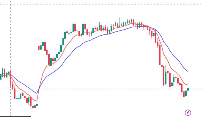
The EMA crossover strategy is a technical strategy used by traders to identify trends based on the crossover of two Exponential Moving Averages with different time periods.
In EMA crossover strategy we use two Ema:
Fast EMA: This is calculated using a shorter time period, reacting fast to recent price changes.
Slow EMA: This is computed using a longer time period, providing a smoother representation of overall trends.
Signals:
Buy Signal: Generated when the Fast EMA crosses above the Slow EMA, indicating a potential upward trend.
Sell Signal: This occurs when the Fast EMA crosses below the Slow EMA, signaling a potential downward trend.
As You can see in above chart red line is our Fast EMA and Blue line is our Slow EMA.
Data Collection:
Before we embark on the exploration of the EMA crossover strategy through backtesting, it’s essential to gather OHLC (Open, High, Low, Close) data for the specific symbol we intend to analyze. This data forms the foundation of our backtesting endeavour, and you can source it from various providers such as Yahoo Finance or your broker’s API. Ensuring access to accurate and comprehensive OHLC data is the first step towards a thorough and insightful evaluation of the strategy’s historical performance.
Don’t forget to store your data in the pandas dataframe because we will be using the pandas module extensively for our backtesting purposes. you can install pandas using the below code.
					!pip install pandas
import pandas as pd
In below code i am using my broker Api to fetch India Nifty 50 OHLC data.
data = historical_data('NIFTY 50',"2020-10-01 09:15:00", "2024-01-09 15:30:00", "day")
data["EMA8"] = ta.ema(data.close, length=8)
data["EMA21"] = ta.ema(data.close, length=21)
In the above code, I am using my broker API to fetch India Nifty 50 OHLC data. and storing it in a data variable. We will use the Pandas_ta module to calculate our fast and slow Ema which are 8 and 21 respectively and store them in their name columns in our dataframe. after all this our data will look like this.
					Date                        Open	     High         Low        Close  Volume	    EMA8          EMA21
2020-11-02 00:00:00+05:30	11697.35	11725.65	11557.40	11669.15	0	11740.538470	11801.719048
2020-11-03 00:00:00+05:30	11734.45	11836.20	11723.30	11813.50	0	11756.752143	11802.790043
2020-11-04 00:00:00+05:30	11783.35	11929.65	11756.40	11908.50	0	11790.473889	11812.400039
2020-11-05 00:00:00+05:30	12062.40	12131.10	12027.60	12120.30	0	11863.768581	11840.390945
2020-11-06 00:00:00+05:30	12156.65	12280.40	12131.85	12263.55	0	11952.608896	11878.859950
...	...	...	...	...	...	...	...
2024-01-03 00:00:00+05:30	21661.10	21677.00	21500.35	21517.35	0	21571.648497	21230.260392
2024-01-04 00:00:00+05:30	21605.80	21685.65	21564.55	21658.60	0	21590.971053	21269.200357
2024-01-05 00:00:00+05:30	21705.75	21749.60	21629.20	21710.80	0	21617.599708	21309.345779
2024-01-08 00:00:00+05:30	21747.60	21763.95	21492.90	21513.00	0	21594.355328	21327.859799
2024-01-09 00:00:00+05:30	21653.60	21724.45	21517.85	21551.95	0	21584.931922	21348.231635
Data Visualization:
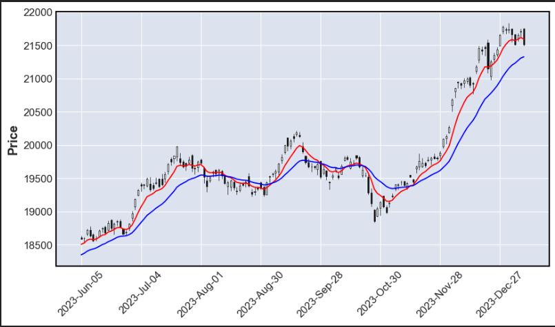
Data visualisation is an important part of our backtesting framework to check whether whatever we are seeing in the charts is truly making sense in our code or not.
Here we will use a fraction of our data store it in dfx and use the mpl-finance library to visualise our chart in the code.
					dfx =data[-150:-1]
import mplfinance as mpf
adp= [mpf.make_addplot(dfx['EMA8'],type ='line'),
     mpf.make_addplot(dfx['EMA21'],type ='line')]
mpf.plot(dfx,type='candle',figratio=(15,8),addplot=adp)
Signal generation:
https://youtu.be/0sbUVne831I?si=rN2qKndcgyJTJbmV
In this part we will do two things first is to generate our signal based on crossover as we talked about earlier.
the second thing we will do is to shift up our close price with one row to calculate our MTM(Mark To Market) on each candle. and we will drop the last value as it will become Nan because of shifting.
					dfx['Signal'] = 0  # Initializing the 'Signal' column with 0
# Adding Long signals where EMA8 crosses above EMA21 and comparing with the previous bar
dfx.loc[(dfx['EMA8'] > dfx['EMA21']) ,'Signal'] = 1
# Adding Short signals where EMA8 crosses below EMA21 and comparing with the previous bar
dfx.loc[(dfx['EMA8'] < dfx['EMA21']), 'Signal'] = -1
dfx['Close_Shifted'] = dfx['Close'].shift(-1)
dfx = dfx.dropna(subset=['Close_Shifted'])
After all this our Dataframe will look like this.
Date         Open        	High	        Low	        Close	        Volume	        EMA8	  EMA21	     Signal Close_Shifted
2024-01-03 00:00:00+05:30	21661.10	21677.00	21500.35	21517.35	0	21571.648497	21230.260392	1	21658.6
2024-01-04 00:00:00+05:30	21605.80	21685.65	21564.55	21658.60	0	21590.971053	21269.200357	1	21710.8
2024-01-05 00:00:00+05:30	21705.75	21749.60	21629.20	21710.80	0	21617.599708	21309.345779	1	21513.0
MTM Calculation:
We will use the following code to calculate MTM on every candle close and in the new column we will calculate the cumulative sum of our MTM to fetch the actual equity of our strategy. Do keep in mind that calculation of MTM will be different for Long and Short Positions.
					# Initializing a new column 'MTM' for Mark-to-Market
dfx['MTM'] = 0
lot =50
# Running a for loop to calculate MTM
for i in range(1, len(dfx)):
    if dfx['Signal'][i] == 1:
        # Long position, subtract 'Close' from 'Close_Shifted' (handle NaN)
        dfx.at[dfx.index[i], 'MTM'] = (dfx['Close_Shifted'][i] - dfx['Close'][i] if not pd.isna(dfx['Close_Shifted'][i]) else 0)*lot
    elif dfx['Signal'][i] == -1:
        # Short position, subtract 'Close_Shifted' from 'Close' (handle NaN)
        dfx.at[dfx.index[i], 'MTM'] = (dfx['Close'][i] - dfx['Close_Shifted'][i] if not pd.isna(dfx['Close_Shifted'][i]) else 0)*lot
dfx['Cumulative_PNL'] = dfx['MTM'].cumsum()
Result:
					Date                        Open	    High	    Low	       Close    Volume	   EMA8	           EMA21	 Signal Close_Shifted  MTM Cumulative_PNL
2024-01-01 00:00:00+05:30	21727.75	21834.35	21680.85	21741.90	0	21564.694454	21155.126575	1	21665.80	-3805.0	279700.0
2024-01-02 00:00:00+05:30	21751.35	21755.60	21555.65	21665.80	0	21587.162353	21201.551432	1	21517.35	-7422.5	272277.5
2024-01-03 00:00:00+05:30	21661.10	21677.00	21500.35	21517.35	0	21571.648497	21230.260392	1	21658.60	7062.5	279340.0
2024-01-04 00:00:00+05:30	21605.80	21685.65	21564.55	21658.60	0	21590.971053	21269.200357	1	21710.80	2610.0	281950.0
2024-01-05 00:00:00+05:30	21705.75	21749.60	21629.20	21710.80	0	21617.599708	21309.345779	1	21513.00	-9890.0	272060.0
Performance Metrics:
Now we Are almost Done with our backtesting part and we can proceed further to analyze our strategy by plotting commutative sum with our close prices so we can check how our strategy performed with the past market conditions. we will again use mpl-finance library to plot our chart.
					dfx.index = pd.to_datetime(dfx.index)
cpd= [
     mpf.make_addplot(dfx['Cumulative_PNL'],type ='line',color='red')]
mpf.plot(dfx,type='line',figratio=(15,8),addplot=cpd)
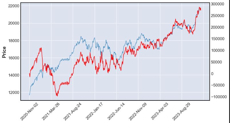
Here, we’ve plotted a chart between our daily close price and cumulative P&L. In 2020, our strategy experienced a significant drawdown. However, since August 2021, our strategy has been aligned with our instrument, yielding nearly 300,000 in profits (excluding costs). While this seems positive on its own, considering other metrics such as drawdowns and maximum loss, I would personally choose to discard this strategy without hesitation.
Conclusions:
In this blog, we delved into backtesting an EMA crossover strategy using Python, examining its performance. Stay tuned for our upcoming post where we explore additional metrics such as drawdowns, time-based drawdowns, and various ratios to gain a comprehensive understanding. If you’re intrigued by algo trading and backtesting, explore more blogs on the subject. To sum up, this blog provided insights into backtesting an EMA crossover strategy using Python. you can checkout my kotak Neo Integration Blog [here] also to learn how to setup your ema crossover trading bot.
Feel free to reach us using our social media handles for any queries regarding trading and Investing.

